ScalableDesktop Classic test

After using ScalableDesktop Classic

Without using ScalableDesktop Classic

Buying air miles is a bad idea

For United Airlines, a saver award round trip ticket from Boston to Shanghai requires 65,000 miles. The round trip usually costs around $1000. This means 1 mile is worth $0.015. When I buy miles, each mile costs $0.035. So it's not worth it to buy miles.

I made the mistake by considering how much it costs to earn miles through taking flights. But earning miles this way is basically free because I'm taking the flight anyways.

So in conclusion, it is almost always a bad idea to buy air miles.

Law of total probability

If \(\{B_n:n=1, 2, 3, \ldots\}\) is a finite partition of a sample space (i.e., a set of pairwise disjoint events whose union is the entire sample space), then for any event A of the same probability space:
$$Pr(A) = \sum_n Pr(A\cap B_n)$$
or, alternatively,
$$Pr(A) = \sum_n Pr(A|B_n)Pr(B_n)$$

Decision Tree

Decision trees are classifiers for instances represented as feature vectors. Nodes are tests for feature values. There is one branch for each value of the feature. Leaves specify the category.

The central choice in the algorithm to build a decision tree is selecting which attribute to test at each node in the tree. We would like to select the attribute that is most useful for classifying examples. A good quantitative measure of the worth of an attribute is information gain, which measures how well a given attribute separates the training examples according to their target classification.

Information gain is related to entropy, that characterizes the (im)purity of an arbitrary collection of examples. Given a collection S, containing positive and negative examples of some target concept, the entropy of S relative to this boolean classification is

$$Entropy(S)\equiv -p_\oplus \log_2 p_\oplus-p_\ominus\log_2 p_\ominus$$

where \(p_\oplus\) is the proportion of positive examples in S and \(p_\ominus\) is the proportion of negative examples in S.

Information gain  is simply the expected reduction in entropy by partitioning the examples according to this attribute. Gain(S, A) of an attribute A, relative to a collection of examples S, is define as

$$Gain(S, A) \equiv Entropy(S) - \sum_{v\in Values(A)}\frac{|S_v|}{|S|}Entropy(S_v)$$

Kinect depth variance analysis

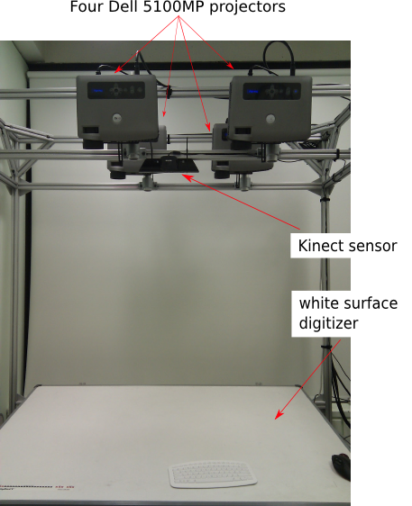
Here are the visualizations of absolute depth differences for each pixel for 40 frames using a Kinect. The setup is like this.

White color shows all pixels with absolute difference greater than 4mm

The high variance at the bottom right corner is due to the mouse which has a shiny surface and the Kinect does not work very well with shiny surfaces.  

White color shows all pixels with absolute difference greater than 2mm

White color shows all pixels with absolute difference greater than 1mm

Absolute depth variance shown as a heat map. The color changes from black, red, yellow and white as the value increases. The difference values are clipped between 0.8 and 2.

Music I like

One of the Pandora stations I listen all the time is based on Lux Aeterna by Clint Mansell on Requiem For A Dream. The music is usually instrumental with electronic string ensembles and has classical influences .

A review of smoothing techniques

Recently I need to smooth the Kinect-based finger tracking result. Without smoothing, there are a lot of jitters as shown in this demo video:

In searching for the best solution, I think it's good to have a review of different smoothing techniques. 

Simple moving average

$$s_t = \frac{1}{k}\sum_{n=0}^{k-1}x_{t-n}=\frac{x_t + x_{t-1} + ...+x_{t-k+1}}{k}=s_{t-1}+\frac{x_t-x_{t-k}}{k}$$

- Disadvantage: cannot be used on the first k-1 terms.

Weighted moving average

Give more weight to the recent terms in the time series. 

- Disadvantage: same as the simple moving average method, it cannot be used on the first k-1 terms. It also requires more complicated calculation at each step as it cannot be written as a inductive formula.

Exponential moving average

$$s_1 = x_0$$

$$s_t = \alpha x_{t-1} + (1 - \alpha)s_{t-1}$$

Exponential smoothing and moving average smoothing are similar in that they both assume a stationary, not trending, time series, therefore lagging behind the trend if one exists. Exponential smoothing also take into account all past data, whereas moving average only takes into account k past data points.

Double exponential smoothing

Double exponential smoothing can be used when there is a trend in the data.

Let {\(x_t\)} be the raw data sequence, {\(s_t\)} be the smoothed value for time t, and {\(b_t\)} be the best estimate of the trend at time t. The output of the algorithm is now written as \(F_{t+m}\). The formulae are:

$$s_1 = x_0$$

$$b_1 = x_1 - x_0$$

And for t>1

$$s_t = \alpha x_t + (1 - \alpha)(s_{t-1} + b_{t-1})$$

$$b_t = \beta(s_t - s_{t-1}) + (1 - \beta)b_{t-1}$$

where \(\alpha\) is the smoothing factor, \(0 < \alpha < 1\), and \(\beta\) is the trend smoothing factor, \(0 < \beta < 1\).