Algorithm complexity

http://bigocheatsheet.com

Shortest path

Dijkstra: \(\Theta(V)\) inserts into priority queue, \(\Theta(V)\) EXTRACT_MIN operations, \(\Theta(E)\) DECREASE_KEY operations.
Min-heap implementation: \(\Theta((V + E)\log V)\)
Fibonacci heap implementation: \(\Theta(\log V)\) for exact min, \(\Theta(1)\) for decrease key and insertion, total amortized cost \(\Theta(V\log V + E)\)

Fibonacci heap

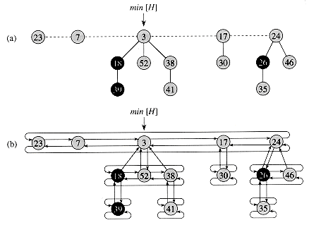
A list of heap-ordered trees. We access the heap by a pointer to the tree root with the overall minimum key.

Main operations

Inserting a node: create a new tree containing only x and insert it into the root list of H.
Decrease-key: cut the node from its parent, then insert the node into the root list with a new key. \(O(1)\)
Delete-min: remove the root of the smallest key, add its children to the root-list, and scan through the linked list of all the root nodes to find the new root of minimum key. We also need need to consolidate the root list by merging roots with the same degree (same number of children). We can think of consolidation as allocating buckets of size up to the maximum possible rank for any root node, which is O(log n). We put each node into the appropriate bucket and march through the buckets, starting at the smallest one, and consolidate everything possible. Therefore the cost of delete-min operation is O(# of children) of the root of the minimum key plus O(# of root nodes).

Population control for roots

We want to make sure that every node has a small number of children. This can be done by ensuring that the total number of descendants of any node is exponential in the number of its children. One way to do this is by only merging trees that have the same number of children (degree).

Let \(s_k\) be the minimum size of any node of degree k in any Fibonacci heap. Let \(y_1, y_2, \ldots, y_k\) denote the children of x in the order in which they were linked to x
\begin{align}
size(x) &\ge s_k \\
& \ge 2 + \sum_{i = 2}^k s_{y_i.degree} \\
& \ge 2 + \sum_{i = 2}^k s_{i - 2} \\
& \ge 2 + \sum_{i = 2}^k F_i \; \text{(by induction)}\\
& = 1 + \sum_{i = 0}^k F_i \\
& = F_{k + 2}\\
&\ge \phi^k
\end{align}

Fibonacci numbers

\begin{align}
F_0 &= 0, \\
F_1 &= 1, \\
F_i &= F_{i - 1} + F_{i - 2} \;\text{for } i \ge 2.
\end{align}

Fourier transformation

The convolution integral

• The output y(t) to an input x(t) is seen as a weighted superposition of impulse response time-shifted by \(\tau\).
• The expression is called the convolution integral and denoted by the same symbol * as in the discrete-time case\[y(t) = \int_{-\infty}^\infty x(\tau)h(t-\tau)d\tau = x(t)*h(t)\]

Harmonic signals (complex exponential) are eigenfunctions for LTI systems. That is,
\[\mathcal{H}f = \lambda f\].

Suppose the input is \(x(t) = Ae^{st}\). The output of the system with impulse repose h(t) is then
\begin{align}\int_{-\infty}^\infty h(t-\tau)Ae^{s\tau}d\tau & = \int_{-\infty}^{\infty}h(\tau)Ae^{s(t-\tau)}d\tau = Ae^{st}\int_{-\infty}^{\infty}h(\tau)e^{-s\tau}d\tau \\ & =Ae^{st}H(s)\end{align}
where H(s) is a scalar dependent only on the parameter s.

Fourier series
Continuous time
\[X[k] = \frac{1}{T}\int_0^Tx(t)e^{-jk\omega_0t}dt\]

Discrete time
\[X[k] = \frac{1}{N}\sum_{n=<N>}x[n]e^{-jk\Omega_0n}\]

Junction tree algorithm for DBN

A naïve approach to do inference on dynamic Bayesian network (DBN) is to unroll DBN for desired number of timesteps and treat it as a static BN. The problems with this are

• Typically the number of timesteps are unknown, and one may use a time window with a fixed length or do some kind of segmentation.
• Space requirement is high
• Dynamic filtering requires rebuilding the entire time history of the process on every timestep. (?)

Understanding the 2TBN (2 time-slice Bayes net) junction tree algorithm implementation

First of all, a junction tree is a clique tree that satisfies the junction tree property. A clique tree comes from the definition of a clique graph. A clique graph of G is a graph where the set of nodes is precisely the set of maximal cliques in G. And if the clique graph is also a tree, it is a clique tree. The junction tree property means that all the maximal cliques containing the same node v must form a connected subtree.

This is one of the algorithm in Kevin Murphy's Bayesian Network Toolbox. The file name is jtree_2TBN_inf_engine.m.

In the constructor of jtree_2TBN_inf_engine, it creates two jtree_engines. It creates one engine just for slice 1. And another engine for 1.5 slice. The 0.5 slice means the interface nodes from the previous slice. Interface nodes are nodes with children in the next slice. In the case of one-level AHMM, the interface nodes include \(G_t, S_t, F_t^G\). So in this case, the interface algorithm (Murphy, 2002) is the same as the frontier algorithm (Zweig, 1996). In the frontier algorithm, the frontier is the full set of hidden nodes.  It also always makes the interface nodes a clique.

One-level AHMM

Resources: http://ttic.uchicago.edu/~kgimpel/papers/jt-dbn.pdf

Computational complexity

http://courses.csail.mit.edu/6.006/fall11/lectures/lecture23.pdf

NP = {decision problems with solutions that can be "checked" polynomial time}

• It is based on the nondeterministic model where an algorithm makes guesses and then says YES or NO.
• Examples: Tetris

NP-hard = "as hard as" every problem in NP

NP-complete = NP \(\cap\) NP-hard

• Tetris is also NP-complete
• Other examples: knapsack, 3-Partition (given n integers, can you divide them into triples of equal sum?), traveling salesman problem, longest common subsequence of k strings, minesweeper, Sudoku, most puzzles, SAT, 3-coloring a given graph, find largest clique in a give graph

Graphical model

Graphical model is a method of using graphs (nodes and edges) to represent dependence or independence relationships among the random variables.

Approximate inference in Bayesian networks
Gibbs sampling

Matlab style guide

Here are some Matlab style guide combined from various sources. I added some changes based on personal preferences and consistency.

1. Kevin Murphy's style guide
2. http://www.datatool.com/downloads/matlab_style_guidelines.pdf

 Names

• Capitalize constants.
• Use camel back notation for vairables, as in hiddenMarkovModel. CamelBack always starts with a lower case letter, and then uses an upper case letter for each new word. Acronyms, such as GaussianHMM, also follow this convention, so would be written as gaussianHmm.
• Names of functions should be written in lower case. 
• It is clearest to have the function and its m-file names the same. Using lower case avoids potential filename problems in mixed operating system environments. 
• To improve readability, underscore may be used.
• Prefix variables denoting a number of elements with the letter n as in nValue for the number of values. 
• Suffix variables storing indices with Ndx as in dataNdx

Comments

• There is a convention that the first comment line after the function header will be searched by the lookfor command. Also, the first contiguous block of comments after the function header will be returned by the help and doc commands. 
• http://stackoverflow.com/questions/3840657/matlab-m-file-help-formatting

Git submodules

When you clone a git repository with submodules, you should add the --recursive option.

git clone --recursive git://github.com/foo/bar.git

If you forget to do that during the cloning, you can update the submodules by

git submodule update --init

init adds the submodule repository URLs to .git/config, and update checks out a specific commit, rather than the tip of a branch.