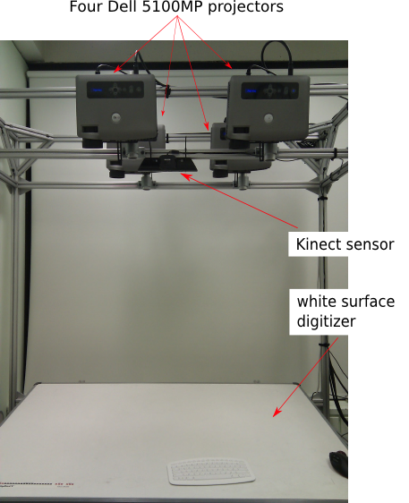
Here are the visualizations of absolute depth differences for each pixel for 40 frames using a Kinect. The setup is like this.
White color shows all pixels with absolute difference greater than 4mm
The high variance at the bottom right corner is due to the mouse which has a shiny surface and the Kinect does not work very well with shiny surfaces.
White color shows all pixels with absolute difference greater than 2mm
White color shows all pixels with absolute difference greater than 1mm
Absolute depth variance shown as a heat map. The color changes from black, red, yellow and white as the value increases. The difference values are clipped between 0.8 and 2.
One of the Pandora stations I listen all the time is based on Lux Aeterna by Clint Mansell on Requiem For A Dream. The music is usually instrumental with electronic string ensembles and has classical influences .
- Disadvantage: cannot be used on the first k-1 terms.
Weighted moving average
Give more weight to the recent terms in the time series.
- Disadvantage: same as the simple moving average method, it cannot be used on the first k-1 terms. It also requires more complicated calculation at each step as it cannot be written as a inductive formula.
Exponential smoothing and moving average smoothing are similar in that they both assume a stationary, not trending, time series, therefore lagging behind the trend if one exists. Exponential smoothing also take into account all past data, whereas moving average only takes into account k past data points.
Double exponential smoothing
Double exponential smoothing can be used when there is a trend in the data.
Let {\(x_t\)} be the raw data sequence, {\(s_t\)} be the smoothed value for time t, and {\(b_t\)} be the best estimate of the trend at time t. The output of the algorithm is now written as \(F_{t+m}\). The formulae are:


